My Bachelor's Degree Thesis

In 2024 I finished my Bachelor’s studies at Technical University of Cluj-Napoca. My diploma project is intitulated Visual-Inertial Odometry based on lane-detection of an autonomous vehicle with constant speed.

Motivation

• I chose this project because of Steven Gong and his experience at F1Tenth; an autonomous racing contest for 1:10 RC Cars.
• Another inspiration for this project was also SPOT by Boston Dynamics. The main attraction was the Real-Time SLAM algorithm it could execute.

Introduction

What is sensor fusion and odometry?

Sensor fusion is collecting and integrating data from multiple sensors in order to get a better understanding of the process that we’re monitoring than if it came from a single source.

Odometry is transforming data coming from sensors that give movement or displacement in order to estimate the ego’s change in position over time.

Why constant speed?

“The linear acceleration signal typically cannot be integrated to recover velocity, or double-integrated to recover position. The error typically becomes larger than the signal within less than 1 second if other sensor sources are not used to compensate this integration error.” - BNO055 documentation

$$noise=1[mg]=0.001[g]=0.001\times 9.81[m/s^2]=0.00981[m/s^2],$$ $$displacement=\frac{1}{2}\times a\times {\text{t}}^2,$$ $$\frac{1}{2}\times a\times t^2\approx 49[m],\text{ where }\text{t}=100[seconds].$$

This right here shows that for 100 [seconds] and a 1 [mg] constant of noise there are 49 [meters] of false displacement. My setup did not allow me to add different movement sensors and so I considered constant speed because the BLDC Motor was in a close loop with the ESC, assuring a Adaptive Cruise Control behaviour.

I will further touch on the connections between the components that I used:

Here, the NUCLEO took care of the real-time algorithms:

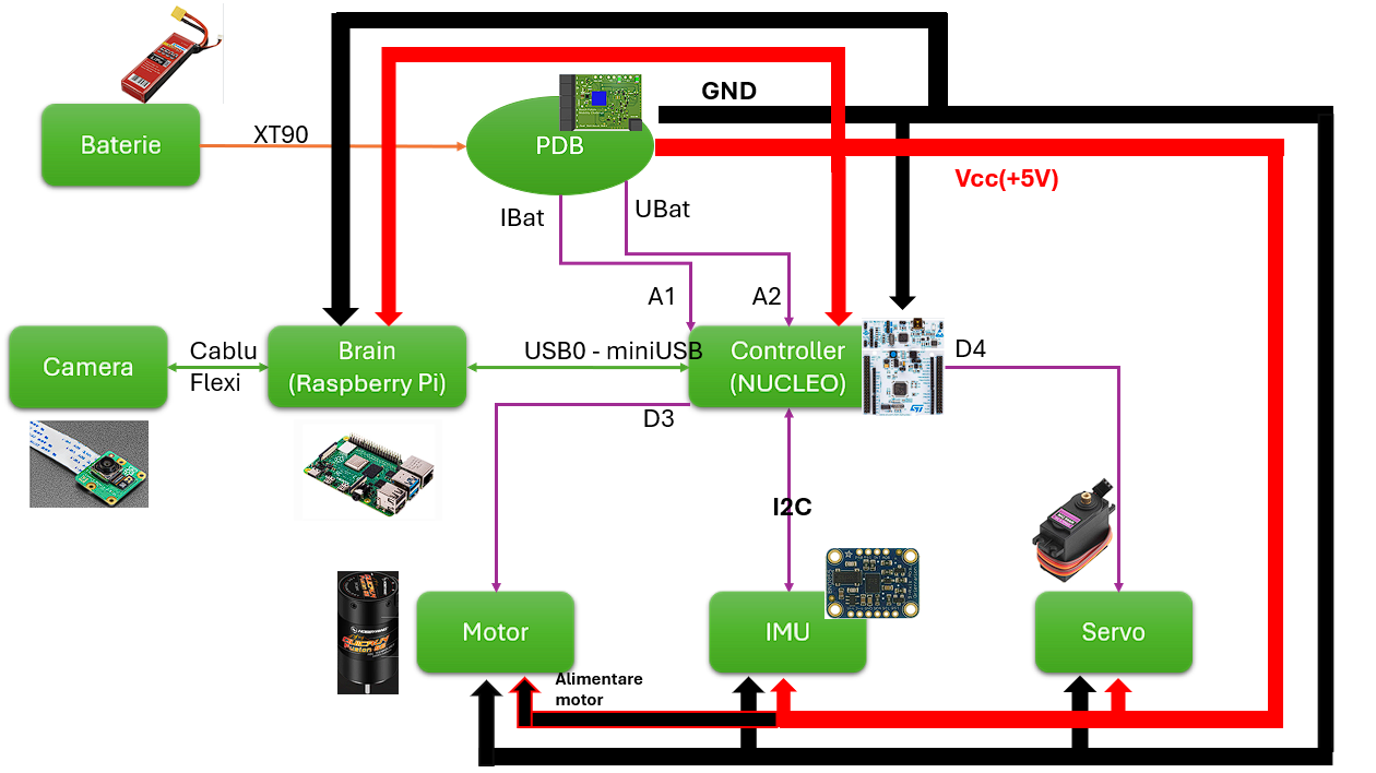
• control of the servomotor and the BLDC Motor,
• Inertial Odometry
• Kalman Filter

and the Raspberry Pi 4B executed all of the perception algorithms:

• Lane-Detection
• Visual Odometry

Control of the servomotor in closed-loop

The main goal of this was to position the ego on the middle of the lane. As error; it would always get the lateral error in [cm] to the middle line generated by the lane-detection algorithm. The proposed control loop was Proportional-Derivative as it gave the best results when testing.

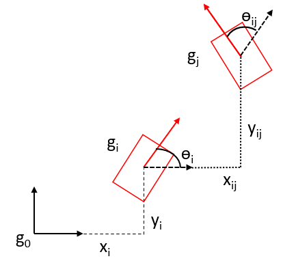
Kinematic Model

In order to get displacement; I needed a Kinematic Model. It was very simplified; as in decomposing the speed vector in the X and Y axis by using the cosinus and sinus trigonometrical functions. The Yaw was updated through a common technique found in the Bicycle Kinematic Model. I can use these formulas because of the constant speed.

$$\Delta x=v\cdot t\cdot \cos (\psi ),$$ $$\Delta y=v\cdot t\cdot \sin (\psi ),$$ $$const=\frac{360\cdot \Delta t}{2\cdot \pi \cdot L}$$ $$\psi =\psi +const\cdot \tan (\theta )$$

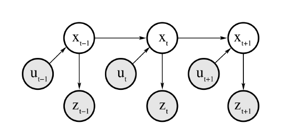
Kalman Filter

It performs the fusion of the two sensors, resulting in visual-inertial odometry

Since the Kalman Filter considers linear processes and this process is clearly nonlinear (trigonometric functions), I can say that I have performed a point-by-point linearization so that the value is considered constant for the entire duration of 100 [ms].

Since this application only approached the Yaw Rate fusion, this Kalman Filter is of 1st order!

I think these next two pictures can perfectly explain the way I implemented the Kalman Filter:

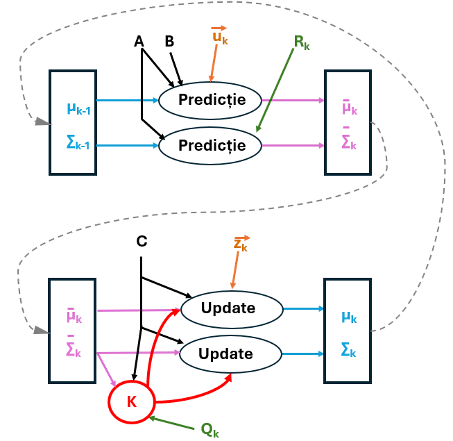
The formula used for the Kalman Gain (for 1st order) is:

$$K=\frac{{\sigma }_{predictie}}{{\sigma }_{predictie}+{\sigma }_{update}}$$

It tells which phase should get more credibility - the prediction or the update.

The results I achieved

In order to test the final algorithm I had three circuits at my disposal. One offered to me by the team that organizes the contest in which this car is actually used - Bosch Future Mobility Challenge, one with the shape of letter "S" and one with a circular shape.

This being covered, here are my results:

$$1st$$

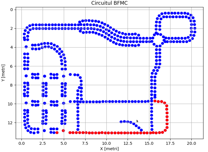
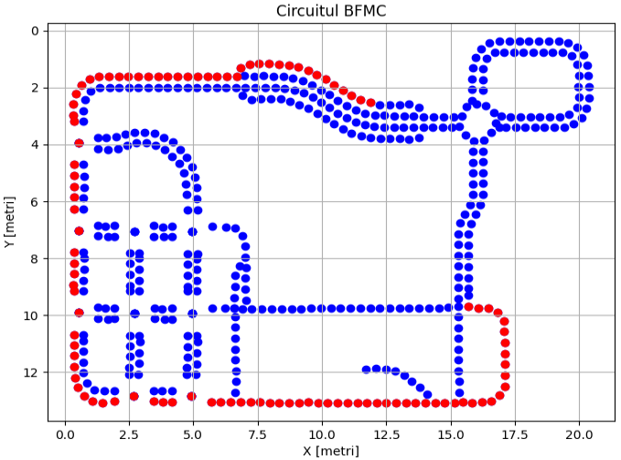
Here I wanted to test the ability of the camera to see two 90 degree' corners one after another. The threshold I used was 7 in order to amplify the corners and as you can see the straight line portion was sacrificed.

$$2nd$$

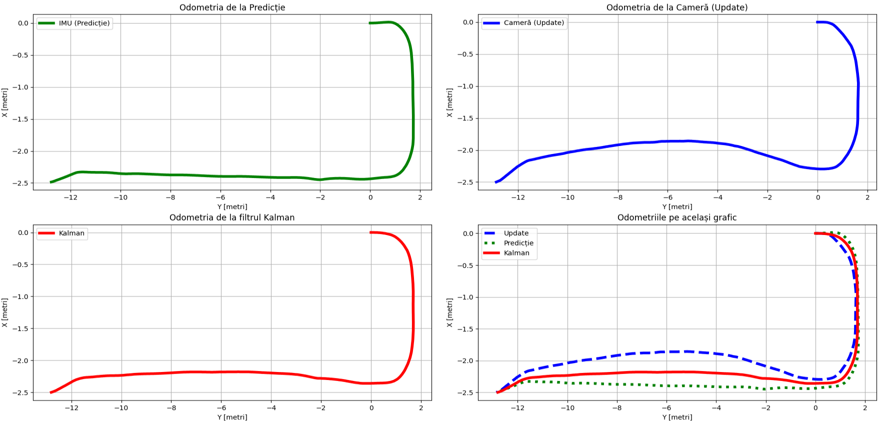
Normally, the IMU's performances should decrease in time and here I was pleasantly surprised to see that it's absolute orientation property could hold on even on longer tracks. Also, the camera held on pretty well in recreating the initial shape of the circuit.

$$3rd$$

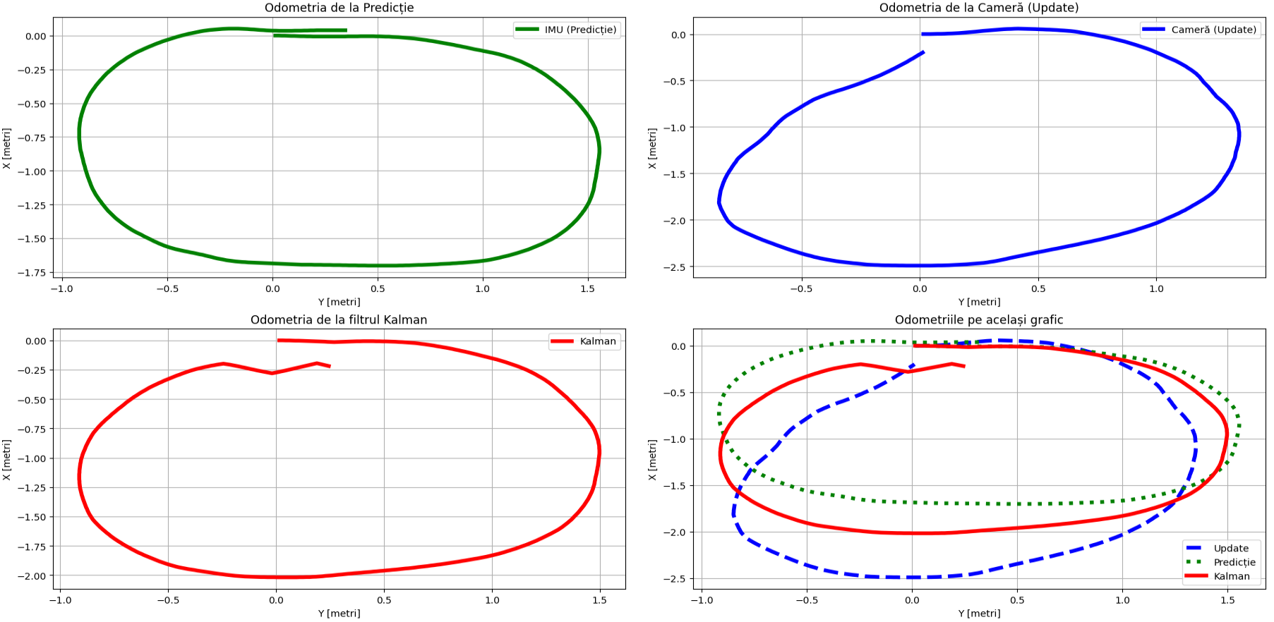
These are probably the most satisfying results I succeeded to collect. Sure, the distance was fairly smaller in comparison with the ones above but I would call these results pretty close to being 1:1. In all these 3 cases the Kalman Gain (K) was ≈ 0.5 so the final result should of course be the mean.

Also, I want to point out that the camera is a sensor that is heavily influenced by environmental factors such as lightning or it’s angle, etc. So when I can control these variables I can get the most out of it.

$$4th$$

In this particular case I wanted to implement a Loop Closure algorithm based on Pose Graphs. Sadly I did not have time to finish it but it would be the first thing I would try to do if I were to start this project again. Maybe I will but now I really want to approach other topics.

Possible issues and bad results

I want to dedicate a small section of this topic to the things that could go wrong with a visual-inertial approach. Firstly, I’ve already mentioned that the camera is a sensor that is highly sensitive to environmental factors such as lightning and angle. In the pictures below, in the first you can see what bad lightning does to the image and how bad it can affect it’s results in the second one. So; if the initial estimation of the camera is bad then it will ruin the whole run, no matter if the next ones are good.

To my surprise, the BNO055 absolute orientation sensor did not fail me at all but then again, I did not have runs longer than 5 minutes. Of course, with time it is destined to suffer drift as well. This is where the loop closure would benefit both downsides.

What would follow?

I would try to implement a SLAM algorithm and I would definitely start with the loop-closure algorithm.