Kalman Filter

The concept of probabilistic or stochastic mathematics deals with the study and modeling of uncertainties. It seeks to combine concepts from probability theory with statistical methods to understand and make decisions under conditions of uncertainty. Stochastic processes represent probabilistic models for phenomena that evolve in space or time. For example, Markov chains model systems where the future depends only on the present state and not on the distant past; a concept known as the Markov property.

To better understand this concept I followed Sebastian Thrun’s infamous book Probabilistic Robotics. You can find the paper here: https://docs.ufpr.br/~danielsantos/ProbabilisticRobotics.pdf

The mathematics behind

Let $X$ be a variable and $x$ an event. If the domain of values that $X$ can take is discrete (such as the outcome of a coin toss - heads or tails), then it is written as:

$$p(X=x)$$

From here on, I will use the notation $p(x)$. As the processes are continuous, the random variables can take on a range of values, and it is considered that all these variables have probability density functions (PDF). An example of such a function is the first-order Gaussian distribution with mean 𝜇 and standard deviation 𝜎:

$$p(x)=\frac{1}{\sqrt{2\pi {\sigma }^2}}\exp \left(-\frac{(x-\mu {)}^2}{2{\sigma }^2}\right)$$

In case of multiple variables, this PDF looks like this:

$$p(x)=\det (2\pi \Sigma {)}^{-\frac{1}{2}}\exp \left(-\frac{1}{2}(x-\mu {)}^{\top }{\Sigma }^{-1}(x-\mu )\right)$$

The Kalman filter is an implementation of the Bayesian filter. This filter is Gaussian and is designed for continuous linear systems. The a priori phase of the Kalman filter is Gaussian if the following properties hold:

1. The state $p(x_t|u_t,x_{t-1})$ has the following linear form:

$$x_t=A_t{x}_{t-1}+B_t{u}_t+{ϵ}_t$$

• Here, $x_t$​ and $x_{t-1}$ represent the state vectors of the system. $A_t$​ is an $n\times n$ matrix where n is the number of states of the system, and $B_t$ is an $n\times m$ matrix where m is the number of control inputs.

• The variable ${ϵ}_t$​ represents a random vector that accounts for the uncertainties of reality (white Gaussian noise with zero mean). This implies that the errors are uncorrelated over time. The covariance of ${ϵ}_t$​ is denoted by $R_t$.

2. The measurement probability $p(z_t|x_t)$, like the state of the system, must also have a linear form with added white noise:

$$z_t=C_t{x}_t+{\delta }_t$$

• $C_t$​ is a $k\times n$ matrix, where k is the dimension of the measurement vector. The vector ${\delta }_t$ also represents white Gaussian noise with zero mean, and its covariance is denoted by $Q_t$​.

3. The assumption $bel(x_0)$ must be normally distributed.

Kalman Filter Algorithm

Input:

• Previous state ( ${\mu }_{t-1}$ )
• Previous covariance ( ${\Sigma }_{t-1}$ )
• Current control inputs ( $u_t$ )
• Current measurements ( $z_t$ )

Output:

• Current estimated state ( ${\mu }_t$ )
• Current covariance ( ${\Sigma }_t$ )

Steps:

1. Prediction of the current state:

   $$\overline{{\mu }_t}=A_t{\mu }_{t-1}+B_t{u}_t$$

2. Prediction of the covariance matrix:

   $$\overline{{\Sigma }_t}=A_t{\Sigma }_{t-1}{A}_t^{\top }+R_t$$

3. Calculation of the Kalman Gain:

   $$K_t=\overline{{\Sigma }_t}{C}_t^{\top }(C_t\overline{{\Sigma }_t}{C}_t^{\top }+Q_t{)}^{-1}$$

4. State update:

   $${\mu }_t=\overline{{\mu }_t}+K_t(z_t-C_t\overline{{\mu }_t})$$

5. Update of the covariance matrix:

   $${\Sigma }_t=(I-K_t{C}_t)\overline{{\Sigma }_t}$$

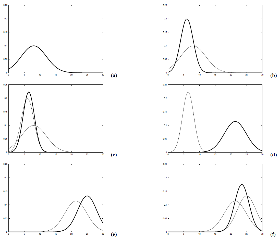
Based on six plots, the functionality of the Kalman filter can be represented as follows:

a) The initial assumption $bex(x_0)$ with its characteristic bell shape.

b) The measurement is taken with added white noise.

c) The prediction phase.

d) The new assumption after applying a control input.

e) A new assumption based on the new measurement with added white noise.

f) The update phase.