Code: GitHub Related to: SeaClear, Line Segment Detector
Final mission
Real-time ground truth validation of 3D pose estimation.
Context
I had to clean up a pool using a mop and constantly throwing out the accumulated water with a bucket that I stole from the cleaning ladies. Not cool.
After it was cleaned, we had to install a metalic grid on it’s bottom that will further be used to detect a reference coordinates point and how far the ROV has displaced from it.
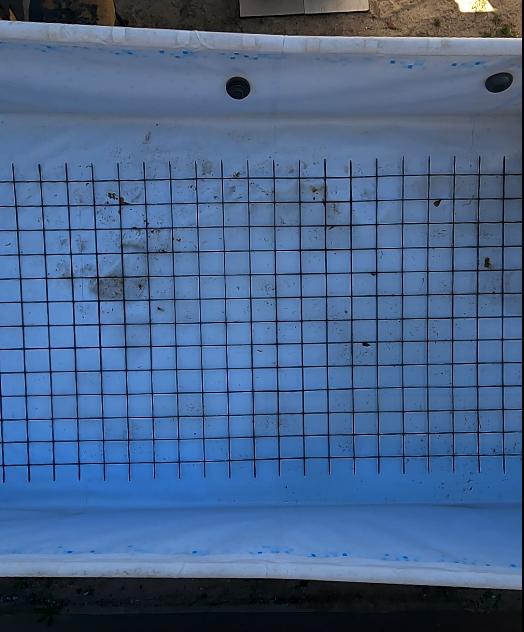
First I had to detect the grid. For the picture above, the boys lend me a GoPro that I attached to an overhead support and shot 1 min worth of full HD video. Should definitely try out the algorithms with 4k.
Preprocessing the data
To make things easier, I applied a region of interest (found empirically) that only has the grid to worry about.
I had to keep it in mind when plotting the lines on the original video because I always had to add up the minimal x and y values.
After applying the ROI, I had to emphasize the vertical and horizontal lines of the grid before applying a detection algorithm. To do that, I:
- transformed the original frame into a gray image (
BGR2GRAY) - applied a
Gaussian Blurto remove the background noise - detected the edges of the frame through
Canny - Apply Dilation and Erosion — Morphological operations apply a structuring element to an input image and generate an output image. I used a kernel of . They help in:
- Removing noise,
- Isolation of individual elements and joining disparate elements in an image,
- Finding of intensity bumps or holes in an image.
gray = cv2.cvtColor(roi_frame, cv2.COLOR_BGR2GRAY)
blur = cv2.GaussianBlur(gray, (5,5), 0)
edges = cv2.Canny(blur, 50, 150, apertureSize=3)
kernel = np.ones((3,3), np.uint8)
edges = cv2.dilate(edges, kernel, iterations=2)
edges = cv2.erode(edges, kernel, iterations=2)
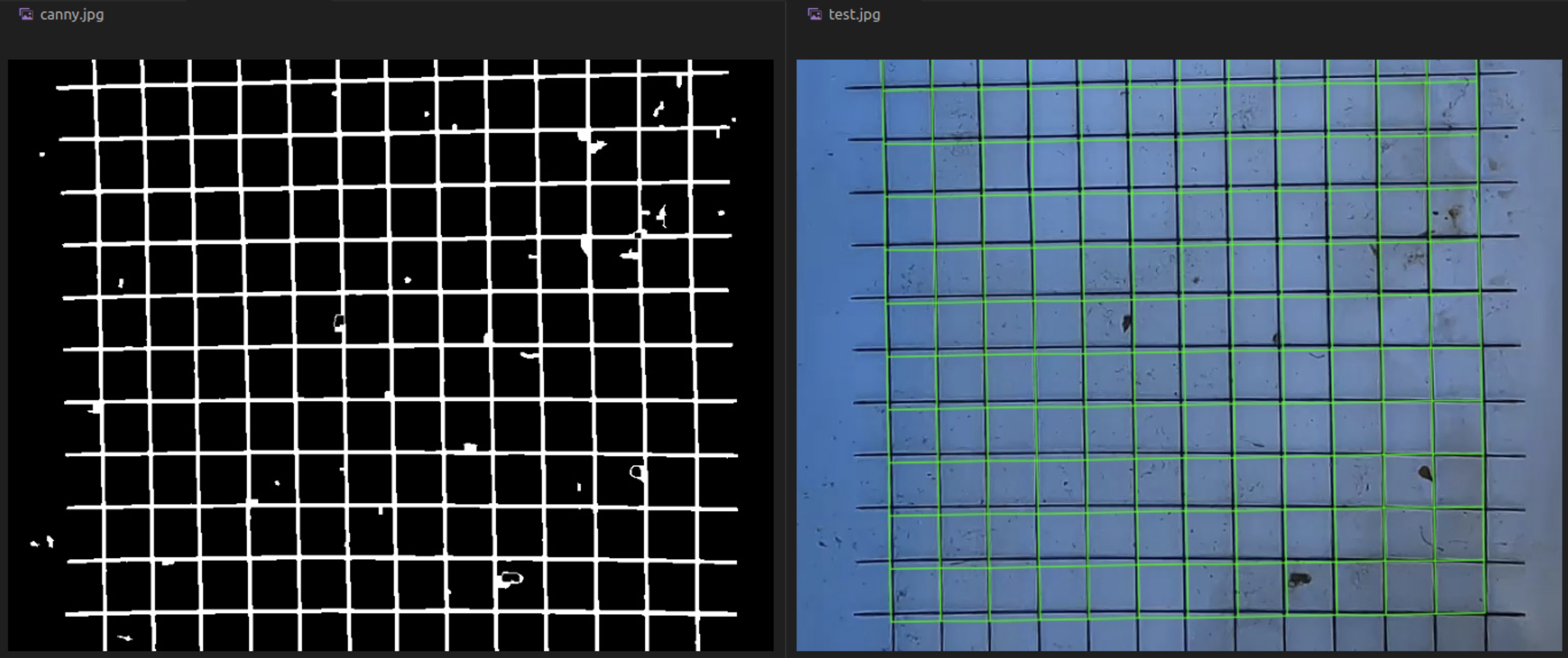
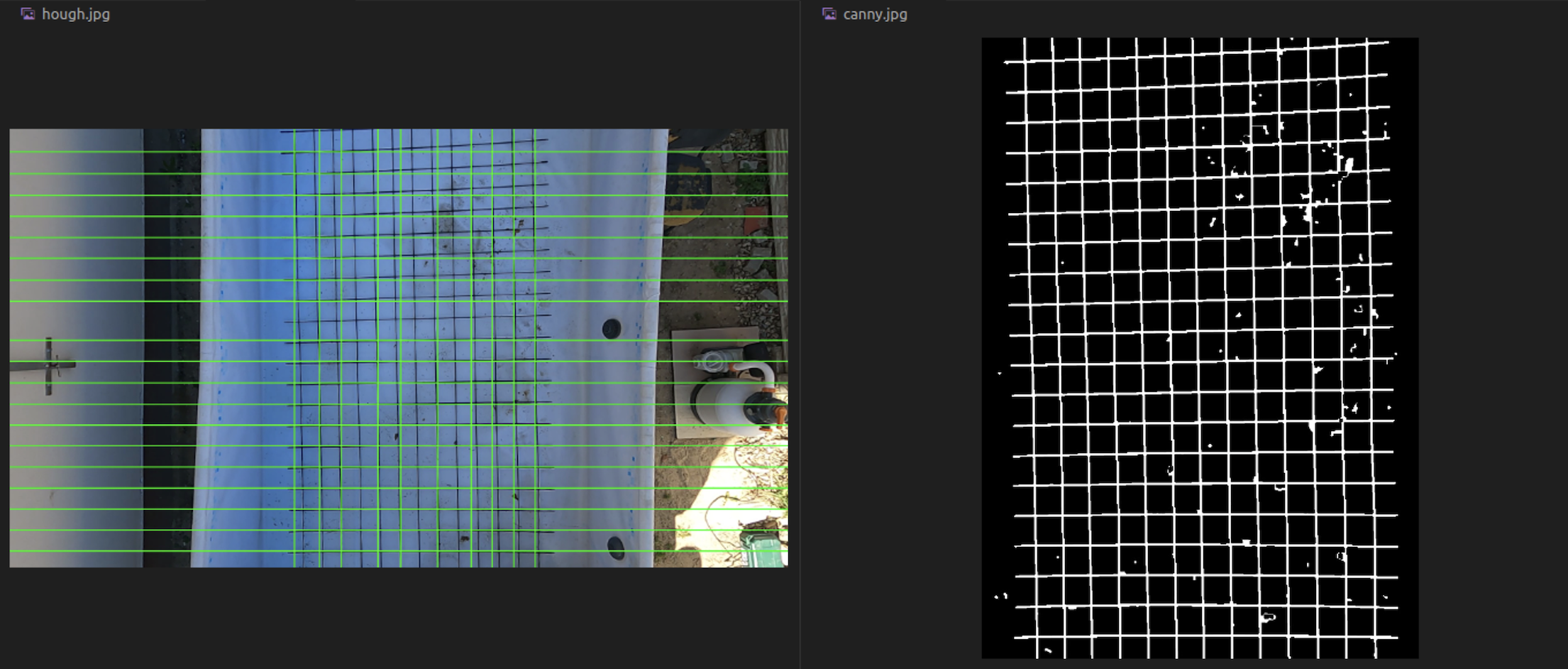
cv2.imwrite('canny.jpg', edges)Postprocessing the data
Hough Transform
I tried to make it work with Probabilistic Hough transform, but it would not be consistent in the output results, no matter how good the preprocessing was
Line Segment Detector
So I tried a technique many people recommended - and that’s Line Segment Detector. It is aimed at detecting locally straight contours on images called line segments. Contours are zones of the image where the gray level is changing fast enough from dark to light or the opposite. I dedicated a whole page to this subject - Line Segment Detector.
I filtered the background noise and actual dirt from the pool with constraining that a segment should at least have a minimal length of 40px.
lsd = cv2.createLineSegmentDetector(0)
# Use cv2.ximgproc.createFastLineDetector() for OpenCV newer than 4.1.0!
lsd_lines = lsd.detect(edges)[0]
horizontal_lines, vertical_lines = self.computeGridLines(lsd_lines)
After sorting the LSD lines into horizontal and vertical, I get the width and height of a square on the metalic grid to compute the virtual grid.
self.generalWidth, self.generalHeight = self.getGridSquareParameters(horizontal_lines, vertical_lines)

def getGridSquareParameters(self, horizontal, vertical, iterations=10):
"""
Iterate through ROI to get the most accurate (width,height)[px] possible.
"""
width_list, height_list = [], []
for _ in range(iterations):
_, width = self.simplify_lines(horizontal, 'horizontal')
_, height = self.simplify_lines(vertical, 'vertical')
width_list.append(width)
height_list.append(height)

return np.mean(width_list), np.mean(height_list)
To draw the rectangulars, OpenCV takes arguments as integers. So the final result could be off in the visual, but in calculus we use the float values!
I used linear algebra to overlay the virtual grid on the actual image.
Steps
I promise it makes sense!
- I click on a reference on the metalic grid,
- The algorithm overlays a virtual grid on top of it which will be used further to compute the displacement of the ROV from the reference point (ground truth),
- I can rotate the grid through keys Left Arrow or Right Arrow to fit as best as possible,
- Stream relative position to the chosen reference point.